Minimum, maximum, and saddle point

Multivariate functions: Stationary points

Minimum, maximum, and saddle point

The concepts of local minimum and local maximum are already known to us for functions of a single variable. The function \(f(x)\) has a local minimum in \(x=a\) if the graph near \(x=a\) lies above \(f(a)\), more precisely, if there is an open interval \(\ivoo{c}{d}\) around \(a\) (that is to say, there are numbers #c\lt a# and #d\gt a#) such that \(f(x)\ge f(a)\) for all \(x\) from \(\ivoo{c}{d}\). For the definition in the case of a function of two variables, we replace the open interval by an open disk.

Local extremes

Let #\epsilon# be a positive number. The open disk around a point #p# of #{\mathbb R}^2# of radius #\epsilon# is the subset #S_{p,\epsilon}# of #{\mathbb R}^2# consisting of all points #q\in {\mathbb R}^2# at distance less than #\epsilon# to #p#. In a formula: \[S_{p,\epsilon}=\left\{q\in{\mathbb R}^2\mid \sqrt{(p_1-q_1)^2 + (p_2-q_2)^2}\lt \epsilon\right\}\tiny.\]

Let #f# be a bivariate function with domain #D# and let #p# be a point of #D#.

The point #p# is called a local minimum of #f# if there is an open disk #S# around #p# (a set of the form #S=S_{p,\epsilon}#) for a suitable value of #\epsilon# so #f(q)\ge f(p)# for all #q\in D\cap S#.
The point #p# is called a local maximum of #f# if there is an open disk #S# around #p# so #f(q)\le f(p)# for all #q\in D\cap S#
The point #p# is called a saddle point of #f# if it is a stationary point, but in every open disk around #p# there are points \(q\) and \(r\) such that \(f(q)\gt f(p)\) and \(f(r)\lt f(p)\).

Below you see the graph of the function \[f(x,y)=\tfrac{1}{2}\!\left((1-(x-\tfrac{1}{2})^2-(y-\tfrac{1}{2})^2\right)\]

maximum of f (x, y)

This function has the following partial derivatives: \[f_x(x,y)=\tfrac{1}{2}-x\qquad\text{and}\qquad f_y(x,y)=\tfrac{1}{2}-y\] In the point \(\rv{\tfrac{1}{2},\tfrac{1}{2}}\), both derivatives are zero. This point is a stationary point. The function has a maximum value there.

The notion of saddle point is similar to the notion of inflection point for a stationary point of a function of a single variable.

Here is a generalization of the theorem Local extrema are stationary points for one variable.

If #f# a bivariate differentiable function on a domain #D# and #p# is a local minimum or local maximum of #f#, then #p# is a stationary point of #f#.

The proof is simple: Write #p=\rv{a,b}#. Then #a# is a local minimum or maximum of the differentiable function #f(a,y)# in the variable #y#. The theorem Local extrema are stationary points for the case of one variable gives \[\left.\frac{\partial f(x,y)}{\partial y}\right|_{\rv{a,b}}=\left.\frac{\dd f(a,y)}{\dd y}\right|_{b}=0\tiny.\] Similarly, we have \[\left.\frac{\partial f(x,y)}{\partial x}\right|_{\rv{a,b}}=\left.\frac{\dd f(x,b)}{\dd x}\right|_{a}=0\tiny.\] This means that #p=\rv{a,b}# is a stationary point of #f#.

Saddle points are by definition stationary points that are neither a local minimum nor a local maximum. The definition of a saddle point is even chosen so that a stationary point of #f# is always a local minimum, local maximum, or saddle point.

As with functions of one variable, for differentiable functions of two variables, the requirement that a point is a stationary point is necessary but not sufficient for a point to be a local minimum or a local maximum. We give a counterexample.

Below is the graph of the function \[f(x,y)=\tfrac{1}{2}\!\left((1-(x-\tfrac{1}{2})^2+(y-\tfrac{1}{2})^2\right)\]

saddle point

This function has the following partial derivatives: \[f_x(x,y)=\tfrac{1}{2}-x\phantom{quad}\text{and}\phantom{quad}f_y(x,y)=y-\tfrac{1}{2}\] At the point \(\tfrac{1}{2},\tfrac{1}{2}\) both derivatives are zero again. But the coordinate line in the direction of the \(x\)-axis is a downward parabola, and the coordinate line in the direction of the \(y\)-axis is an upward parabola. Therefore, the point \(\rv{\tfrac{1}{2},\tfrac{1}{2}}\) must be a saddle point.

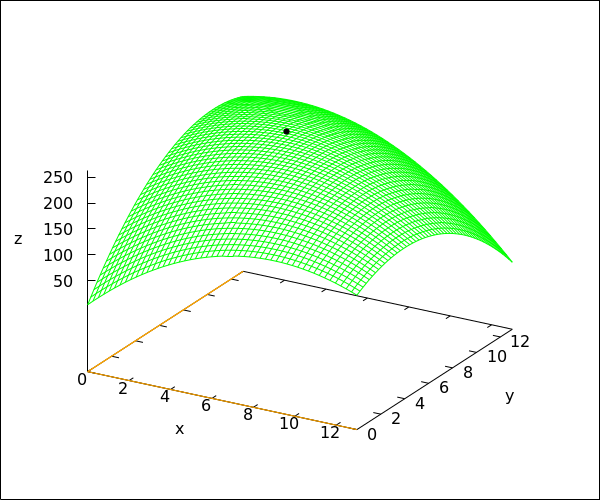
The function \[f(x,y)=-3\cdot x^2+2\cdot y\cdot x-8\cdot y^2+14\] has a local maximum. Which point is it?

#\rv{0, 0}#

Since a local maximum of a multivariate differentiable function is a stationary point, we first calculate the stationary points. The partial derivatives of #f# are \[f_x(x,y)=2\cdot y-6\cdot x\phantom{quad}\text{and}\phantom{quad}f_y(x,y)=2\cdot x-16\cdot y\tiny.\] The stationary points are the solutions of the system of equations \[\lineqs{2\cdot y-6\cdot x&=&0\cr 2\cdot x-16\cdot y&=&0\cr}\]

This system has exactly one solution: #{x = 0\land y = 0}#. We conclude that there is exactly one stationary point: #\rv{0, 0}#. It is given that #f# has a local maximum, so this point must be the answer: #\rv{0, 0}#.

The graph of the function #f# is shown in the figure below. The point #\rv{0,0,14}# corresponding to the local maximum is indicated by a small black disk.

New example